3 Inference for MLM Continued
3.1 Inference for the Covariance \(\Sigma\)
Consider \(b\) partitions of a random vector \(X\), so that we write \(\Sigma\) as
\[\Sigma = \begin{pmatrix} \Sigma_{11} & \Sigma_{12} & \cdots & \Sigma_{1b} \\ \vdots & \ddots & & \vdots \\ \Sigma_{b1} & \cdots & & \Sigma_{bb} \end{pmatrix}\]
Assume \(X \sim \mathcal{MN}(\mathbf{1}_n \mu,\, I_n,\, \Sigma)\), with \(n \geq p + 1\) such that \(\Pr[\hat{\Sigma} > 0] = 1\).
3.2 Testing Mutual Independence
Let
\[X = \begin{pmatrix} X_1 \\ X_2 \end{pmatrix}, \quad \mu = \begin{pmatrix} \mu_1 \\ \mu_2 \end{pmatrix}, \quad \Sigma = \begin{pmatrix} \Sigma_{11} & \Sigma_{12} \\ \Sigma_{21} & \Sigma_{22} \end{pmatrix}.\]
We consider testing
\[H_0 : \Sigma_{12} = \Sigma_{21} = 0\]
Under \(H_0\) it is easy to show that
\[f(x \mid \mu, \Sigma) = f(x_1 \mid \mu_1, \Sigma_{11})\; f(x_2 \mid \mu_2, \Sigma_{22})\]
with restricted MLEs
\[\hat{\Sigma}_{11} = \frac{1}{n} X_1^\top Q_1 X_1, \qquad \hat{\Sigma}_{22} = \frac{1}{n} X_2^\top Q_2 X_2.\]
Without restrictions, under \(H_1 = H_0^c\), the unrestricted MLE is \(\hat{\Sigma} = \frac{1}{n} X^\top Q X\).
The LRT statistic is
\[\Sigma = \frac{f(x_1 \mid \hat{\mu}_1, \hat{\Sigma}_{11})\; f(x_2 \mid \hat{\mu}_2, \hat{\Sigma}_{22})}{f(x \mid \hat{\mu}, \hat{\Sigma})} = \frac{(|\hat{\Sigma}_{11}||\hat{\Sigma}_{22}|)^{-n/2}}{|\hat{\Sigma}|^{-n/2}}.\]
It is useful to work with
\[\Sigma^{2/n} = \frac{|\hat{\Sigma}|}{|\hat{\Sigma}_{11}||\hat{\Sigma}_{22}|} = \frac{|\hat{\Sigma}_{22} - \hat{\Sigma}_{21}\hat{\Sigma}_{11}^{-1}\hat{\Sigma}_{12}|}{|\hat{\Sigma}_{22}|} = \frac{|E|}{|E + H|}.\]
Lemma 3.1 (Null Distribution of the LRT) We can show that
\[\Sigma^{2/n} \xrightarrow{H_0} U(p_1,\, p_2,\, n - p_1 - 1)\]
3.2.1 Testing Block-wise Independence
More generally, consider
\[H_0 : \Sigma = \begin{pmatrix} \Sigma_{11} & & 0 \\ & \ddots & \\ 0 & & \Sigma_{bb} \end{pmatrix}\]
The LRT statistic extends naturally to
\[\lambda^{2/n} = \frac{|\hat{\Sigma}|}{\prod_{j=1}^{b} |\hat{\Sigma}_{jj}|}\]
3.3 Improved Estimation of \(\Sigma\)
3.3.1 Loss Functions and Risk
Consider estimators of the form \(\hat{\Sigma} = \hat{\Sigma}(S)\), with \(S \sim W_p(n, \Sigma)\). We say \(\Sigma \in \mathcal{S}_p^+\), the cone of \(p \times p\) positive definite matrices in \(\mathbb{R}^p\). Assume \(\Sigma > 0\) and \(p \leq n\), so that \(\Pr(S > 0) = \Pr(S\in S^+_p) = 1\).
The loss incurred by an estimate \(\hat{\Sigma}\) is measured by a loss function \(L(\hat{\Sigma}, \Sigma)\), such that \(L \geq 0\) and \(L = 0\) iff \(\hat{\Sigma} = \Sigma\). An estimator \(\hat{\Sigma}(S)\) is evaluated in terms of its risk function
\[R(\hat{\Sigma}, \Sigma) = \mathbb{E}\left[L(\hat{\Sigma}, \Sigma)\right].\]
Two commonly used loss functions are:
(1) Quadratic Loss: \[L_1(\hat{\Sigma}, \Sigma) = \operatorname{tr}\!\left(\Sigma\hat{\Sigma}^{-1} - I\right)^2\]
(2) Stein’s Loss: \[L_2(\hat{\Sigma}, \Sigma) = \operatorname{tr}(\Sigma\hat{\Sigma}^{-1}) - \log|\Sigma\hat{\Sigma}^{-1}| - p\]
\(L_2\) is often preferred to \(L_1\) because:
- \(L_1(\hat{\Sigma}, I) \to p\) as \(\hat{\Sigma} \to 0\) and \(L_1(\hat{\Sigma}, I) \to \infty\) as \(\hat{\Sigma} \to \infty\)
- Whereas \(L_2(\hat{\Sigma}, I) \to \infty\) as \(\hat{\Sigma} \to 0\) or \(\hat{\Sigma} \to \infty\).
3.3.2 Reduction by Invariance
Consider equivariant (Definition 3.2) estimators of \(\Sigma\). We consider invariance with respect to a group \(\mathcal{G}\) of measurable mappings of the sample space \(\mathcal{X}\) onto itself, for which \(g : \mathcal{X} \to g(\mathcal{X})\) is a bijection for all \(g \in \mathcal{G}\).
Let \(GL(p)\) be the general linear group of all \(p \times p\) non-singular real matrices. A natural group of transformations for covariance matrices is \((x \mapsto Ax,\; \Sigma \mapsto A\Sigma A^\top)\).
Definition 3.1 (Invariant Loss Function) If \(\mathcal{G} \subseteq GL(p)\), a loss function \(L\) is \(\mathcal{G}\)-invariant if
\[L(A\hat{\Sigma}A^\top,\, A\Sigma A^\top) = L(\hat{\Sigma},\, \Sigma), \quad \forall A \in \mathcal{G}.\]
Lemma 3.2 (Risk Transformation) If a loss function \(L\) is \(\mathcal{G}\)-invariant, the risk function of any estimator \(\hat{\Sigma}(S)\) transforms as
\[R\!\left(A^{-1}\hat{\Sigma}(ASA^\top)A^{-\top},\, \Sigma\right) = R\!\left(\hat{\Sigma}(ASA^\top),\, A\Sigma A^\top\right) = R\!\left(\hat{\Sigma}(S),\, A\Sigma A^\top\right).\]
Definition 3.2 (Equivariant Estimators) An estimator \(\hat{\Sigma}(S)\) is \(\mathcal{G}\)-equivariant if
\[\hat{\Sigma}(ASA^\top) = A\hat{\Sigma}(S)A^\top, \quad \forall A \in \mathcal{G},\; S \in \mathcal{S}_p^+.\]
3.3.3 Best Fully Equivariant Estimators
Lemma 3.3 (Characterization of \(GL\)-Equivariant Estimators) An estimator \(\hat{\Sigma}(S)\) is \(GL\)-equivariant if and only if
\[\hat{\Sigma}(S) = c\, S \quad \text{for some } c > 0.\]
Proposition 3.1 (Best Fully Equivariant Estimators)
The best fully equivariant estimator of \(\Sigma\) with respect to \(L_1\) is \[\hat{\Sigma}(S) = \frac{1}{n + p + 1} S.\]
The best fully equivariant estimator of \(\Sigma\) with respect to \(L_2\) is \[\hat{\Sigma}(S) = \frac{1}{n} S.\]
3.3.4 Best \(GT\)-Equivariant Estimators
Let \(GT\) be the subgroup of all \(p \times p\) non-singular lower triangular matrices.
Lemma 3.4 (Characterization of \(GT\)-Equivariant Estimators) Let \(S_T\) be the unique lower triangular root of \(S\). An estimator \(\hat{\Sigma}(S)\) is \(G_T\)-equivariant if and only if
\[\hat{\Sigma}(S) = S_T\, \Delta\, S_T^\top\]
for a fixed matrix \(\Delta = \operatorname{diag}(\delta_1, \ldots, \delta_p)\) with each \(\delta_j > 0\).
Stein (1962) derived the improved estimator of \(\Sigma\), by finding the optimal \(GT\)-equivariant estimator with respect to \(L_2\):
\[\hat{\Sigma}(S) = S_T\, \hat{\Delta}\, S_T^\top, \qquad c_i = \frac{1}{n + p + 1 - 2i}.\]
Example 3.1 (Loss and Dimensionality)
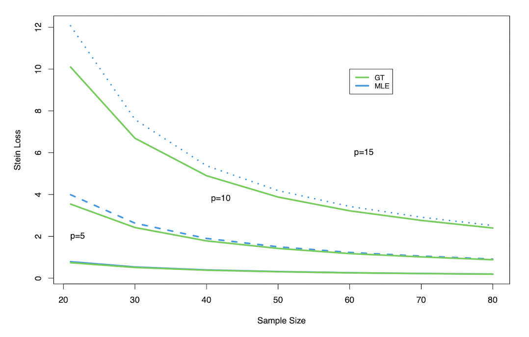
Stein loss as a function of sample size \(n\) for \(p \in \{5, 10, 15\}\) shows that the \(GT\) estimator consistently achieves lower loss than the MLE, with the gap widening as \(p\) increases relative to \(n\).
3.4 Bayesian Analysis of the MNLM
3.4.1 Model and Prior
The Bayesian analysis requires two ingredients:
(i) Sampling model: \[p(Y \mid B, \Sigma) = \mathcal{MN}(XB,\, I_n,\, \Sigma)\]
(ii) Prior distribution: \(p(B, \Sigma)\)
Inference is based on the posterior distribution: \[p(B, \Sigma \mid Y) = \frac{p(Y \mid B, \Sigma)\; p(B, \Sigma)}{p(Y)}.\]
3.4.2 Improper Prior Analysis
Consider the improper prior
\[p(B, \Sigma) = p(B)\, p(\Sigma) \propto |\Sigma|^{-(p+1)/2}.\]
Full conditional for \(B\):
\[p(B \mid Y, \Sigma) \propto \exp\!\left\{-\frac{1}{2}\operatorname{tr}\!\left[\Sigma^{-1}(Y - XB)^\top(Y - XB)\right]\right\}\]
Completing the square in \(B\) gives
\[p(B \mid Y, \Sigma) \propto \exp\!\left\{-\frac{1}{2}\operatorname{tr}\!\left[\Sigma^{-1}(B - \hat{B})^\top X^\top X(B - \hat{B})\right]\right\}\]
which is the kernel of \(\mathcal{MN}\!\left(\hat{B},\, (X^\top X)^{-1},\, \Sigma\right)\).
Definition 3.3 (Inverse Wishart Distribution) Let \(A \sim W_p(\nu, S)\) with \(S > 0\) and \(\nu > p\). Then \(B = A^{-1} \sim \mathcal{IW}_p(\nu, S^{-1})\):
\[p(B) \propto |B|^{-\nu/2} \exp\!\left\{-\frac{1}{2}\operatorname{tr}\!\left(B^{-1} S^{-1}\right)\right\}, \qquad \mathbb{E}(B) = \frac{S^{-1}}{\nu - 2(p+1)} \text{ for } \nu > 2(p+1).\]
Full conditional posterior for \(\Sigma\):
\[p(\Sigma \mid Y, B) \propto |\Sigma|^{-n/2} \exp\!\left\{-\frac{1}{2}\operatorname{tr}\!\left[\Sigma^{-1}Q_B\right]\right\} \cdot |\Sigma|^{-(p+1)/2} \propto |\Sigma|^{-(n+p+1)/2} \exp\!\left\{-\frac{1}{2}\operatorname{tr}\!\left[\Sigma^{-1} Q_B\right]\right\}\]
which is the kernel of an Inverse Wishart.
3.4.3 Marginal Posteriors
\[p(\Sigma \mid Y) = \int p(\Sigma \mid Y, B) dp(B \mid Y) \propto \int p(Y \mid B, \Sigma) p(\Sigma) dp(B \mid Y)\]
Lemma 3.5 (Marginal Posterior \(\Sigma \mid Y\)) \[\Sigma \mid Y \sim \mathcal{IW}\!\left(n - q + p + 1,\; Q\right), \qquad Q = (Y - X\hat{B})^\top(Y - X\hat{B}),\]
with \(\mathbb{E}(\Sigma \mid Y) = \dfrac{Q}{n - q - p - 1}\).
3.5 Some Distribution Theory
Definition 3.4 (Multivariate \(T\) Distribution) The non-central, non-standard \(T\) distribution \(X \sim T_\nu(\theta, \Sigma)\) has the form:
\[f(x) \propto \sigma^{-1} \left[ v + \left( \frac{x - \mu}{\sigma} \right)^2 \right]^{-\frac{(\nu + 1)}{2}}\]
For the generalized vector-valued random quantities such that \(X : p \times 1\), it has the density:
\[f(x) \propto |\Sigma|^{-1/2}\left[v + (x - \theta)^\top \Sigma^{-1}(x - \theta)\right]^{-(\nu + p)/2}\]
Definition 3.5 (Definition (Matrix T)) We say that \(X : p \times q\) has a matrix \(T\) distribution, with df \(\nu\), location \(\theta\) and scales \(\Sigma\), \(\Lambda\), iff
\[f(x) \propto [\Lambda + (x - \theta)^\prime \Sigma^{-1}(x - \theta)]^{-\nu/2}\]
3.5.1 Posterior Marginal \(B \mid Y\)
\[p(B \mid Y) \propto \int p(Y \mid B, \Sigma) p(B \mid \Sigma) dp(\Sigma)\]
Lemma 3.6 Lemma: \(B \mid Y \sim MT_{\nu^*}(\hat{B}, Q, (X'X)^{-1})\) s.t.
\[p(B \mid Y) \propto |Q + (B - \hat{B})' X' X (B - \hat{B})|^{-\nu^*/2}\]
Corollary 3.1 Corollary: Each column of \(B \mid Y\) follows a multivariate T distribution
\[p(B_j \mid Y) \propto [Q_{jj} + (B_j - \hat{B}_j)' X' X (B_j - \hat{B}_j)]^{-\nu^*/2}\]
3.5.2 HPD Regions for \(B \mid Y\)
Let
\[U(B) = \frac{|Q|}{|Q + (B - \hat{B})^\top X^\top X (B - \hat{B})|}.\]
Lemma 3.7 (HPD Region Characterization) \(p(B \mid Y)\) is a monotone increasing function of \(U(B)\). Therefore, a point \(B_0\) lies inside the \((1 - \alpha)\) HPD region if and only if
\[\Pr\{U(B) > U(B_0) \mid Y\} \geq 1 - \alpha.\]
Lemma 3.8 (Distribution of \(U\)) Let \(\theta : p \times q \sim \mathcal{MT}_\nu(\hat{\theta}, A, (X^\top X)^{-1})\). Then
\[U(\theta) \sim U(p, q, \nu).\]
Corollary 3.2 (Duality with Frequentist Testing) The posterior probability \(\Pr\{U(B) > U(B_0) \mid Y\}\) is numerically equivalent to the significance level associated with the null \(H_0 : B = B_0\) against \(H_1 : B \neq B_0\).
3.6 Conditionally Conjugate Priors
The sampling density \(p(Y \mid B, \Sigma)\) can be written as
\[p(Y \mid B, \Sigma) \propto \frac{\exp\!\left\{-\frac{1}{2}\operatorname{tr}\!\left[\Sigma^{-1}Q\right]\right\}}{|\Sigma|^{n/2}} \cdot \exp\!\left\{-\frac{1}{2}\operatorname{tr}\!\left[\Sigma^{-1}(B - \hat{B})^\top X^\top X(B - \hat{B})\right]\right\},\]
suggesting a natural factorization of the prior:
\[p(B, \Sigma) = p(B \mid \Sigma)\; p(\Sigma)\]
where
\[p(B \mid \Sigma) \sim \mathcal{MN}(B_0,\, A,\, \Sigma), \qquad p(\Sigma) \sim \mathcal{IW}(\nu,\, S_0).\]
3.6.1 Common Specifications
Zellner \(g\)-prior:
\[A = g\,(X^\top X)^{-1}, \qquad S_0 = I_p, \qquad B_0 = 0.\]
Empirical Bayes: identify values of \(g\) and \(\nu\) that maximize the integrated likelihood
\[\mathcal{L}(g, \nu) = \int p(Y, B, \Sigma)\, dB\, d\Sigma.\]