6 Generalized Linear Mixed Effects Models (GLMM)

6.1 Linear Mixed Effects Models

\[Y_i = X_i \beta + Z_i b_i + \epsilon_i, \quad b_i \sim N(0, D(\alpha));\]

Inference for LMEM hinges on two essential facts:

6.1.1 (i) Closed form marginal moments

\(E(Y_i) = X_i \beta\)
\(Cov(Y_i) = Z_i D(\alpha) Z_i' + E(\alpha) = V_i(\alpha)\)
\(Cov(Y_i, Y_j) = 0, \quad \text{for any } i \neq j\)

6.1.2 (ii) Convolutions of Normals are Normal

\[Y_i \mid \beta, \alpha \sim N(X_i \beta, V_i(\alpha))\]

6.2 Motivation (Incidence of Bovine Pleuropneumonia)

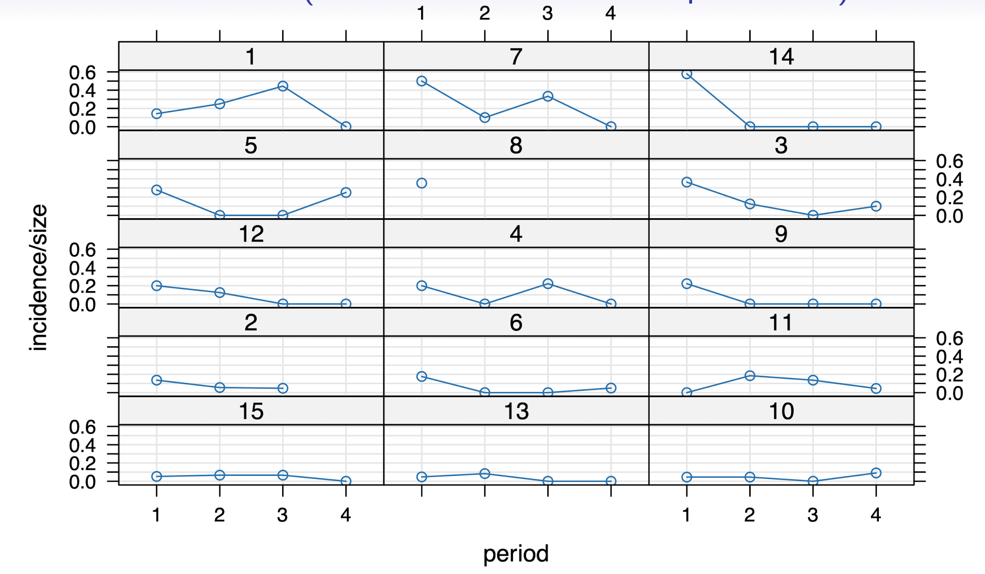
Modeling dependent Binomial observations (no. cases within herd)

6.3 Motivation (Seizure Counts)

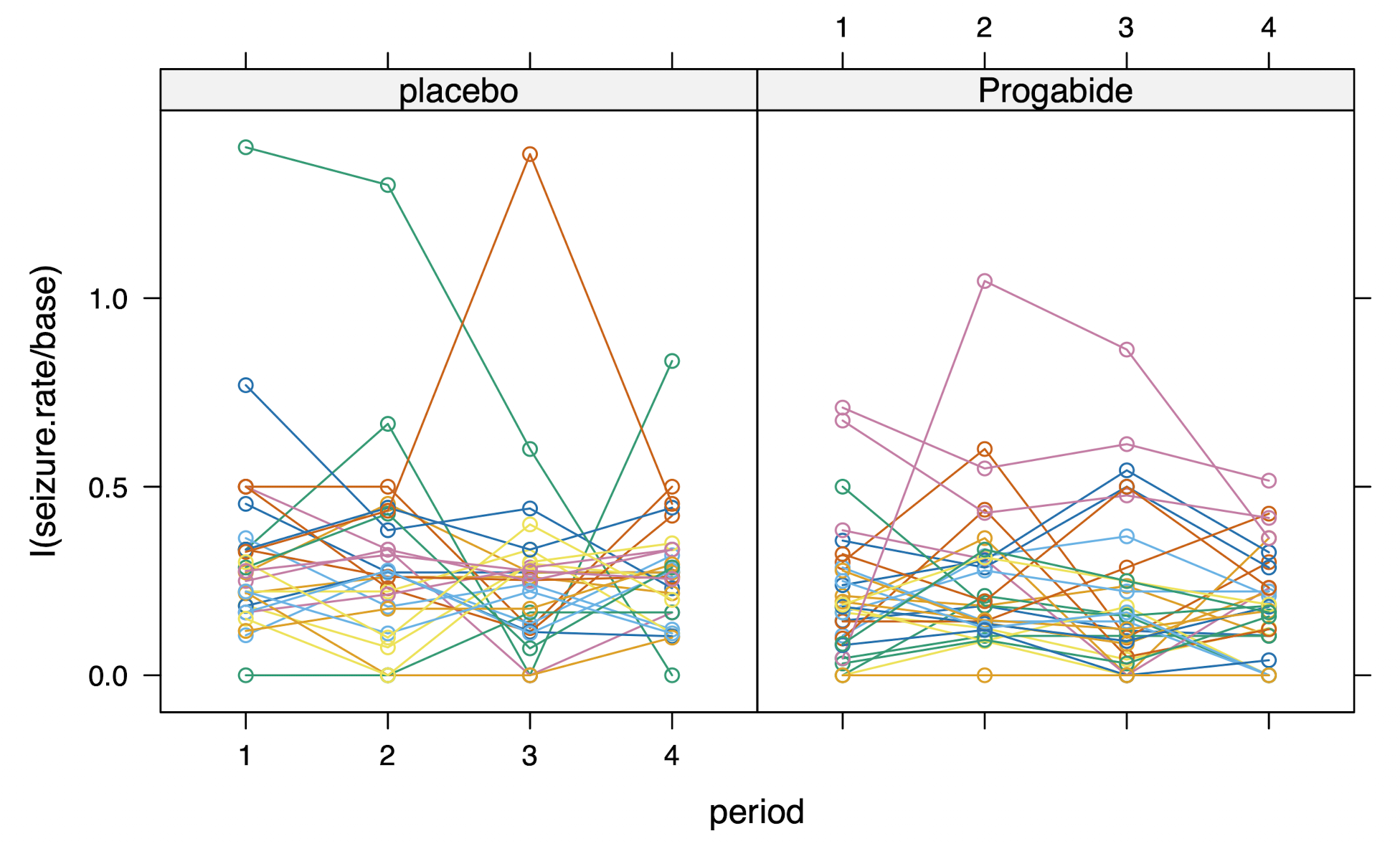
Modeling dependent Counts (no. of seizures in time)

6.4 Generalized Linear Mixed Models (GLMM)

A GLMM is defined as follows:

\(p(y_{ij} \mid \theta_{ij}) = \exp \{ [y_{ij}\theta_{ij} - d(\theta_{ij})] / a(\alpha) + c(y_{ij}, \alpha) \}\)

\(E(y_{ij} \mid \theta_{ij}) = \mu_{ij}\), with \(\eta_{ij} := g(\mu_{ij}) = x_{ij}'\beta + z_{ij}'b_i\)

\(b_i \sim_{iid} N(0, D(\alpha))\)

With Conditional Moments

\[E(y_{ij} \mid b_i) = \frac{\partial d(\theta_{ij})}{\partial \theta_{ij}} = \mu_{ij}\]

\[V(y_{ij} \mid b_i) = a(\alpha) \frac{\partial^2 d(\theta_{ij})}{\partial \theta_{ij}^2} = a(\alpha)V(\mu_{ij})\]

6.5 Marginal Moments

\[E(Y_{ij}) = E\{E(Y_{ij} \mid b_i)\} = E_b \{ g^{-1}(x_{ij}'\beta + z_{ij}'b_i) \}\]

\[Var(Y_{ij}) = E\{Var(Y_{ij} \mid b_i)\} + Var\{E(Y_{ij} \mid b_i)\}\]

\[\begin{aligned} Cov(Y_{ij}, Y_{ik}) &= E\{Cov(Y_{ij}, Y_{ik} \mid b_i)\} + Cov\{E(Y_{ij} \mid b_i), E(Y_{ik} \mid b_i)\} \\ &= Cov\{g^{-1}(x_{ij}'\beta + z_{ij}'b_i), g^{-1}(x_{ik}'\beta + z_{ik}'b_i)\} \end{aligned}\]

\[Cov(Y_{ij}, Y_{i'k}) = 0\]

6.6 Inferential Strategies

(i) Marginal Likelihood

Make specific assumptions about the distribution of the random effects \(b_i\) and carry out inference for the fixed effects by marginalizing over \(b_i\).

(ii) Conditional Likelihood

Treat \(b_i\) as a nuisance parameter and estimate \(\omega\), \(\vartheta\) conditioning on a sufficient statistic for \(b_i\). This is covered for completeness.

6.7 Conditional Likelihood

Consider a sampling model \(p(y \mid \lambda, \phi)\), with \(\theta = (\lambda, \phi)\), and \(\phi\) is a nuisance parameter.

If \(T_1\) and \(T_2\) are sufficient statistics for \(\lambda\) and \(\phi\), respectively, we can write

\[p(y \mid \lambda, \phi) = p(t_1 \mid t_2, \lambda) p(t_2 \mid \lambda, \phi)\]

Inference about \(\lambda\) may be based on the conditional likelihood

\[\mathcal{L}_C(\lambda) = p(t_1 \mid t_2, \lambda)\]

Note that, because \(T_2\) is not assumed ancillary, some information is usually lost. In this sense the conditional likelihood solution is suboptimal, when compared to marginal likelihood calculations.

6.8 Conditional Likelihood Inference for GLMM

Consider \(g(\mu_{ij}) = \theta_{ij} = x_{ij}'\beta + z_{ij}'b_i\) (canonical).

For simplicity, consider \(a(\alpha) = 1\), common for Poisson, Binomial, \(\ldots\)

The likelihood function is

\[\mathcal{L}(\beta, \alpha) = \exp \left\{ \sum_{i} \sum_{j} [y_{ij}x_{ij}'\beta + y_{ij}z_{ij}'b_i - d(x_{ij}'\beta + z_{ij}'b_i)] \right\}\]

with \(E(Y_{ij} \mid b_i) = d'(x_{ij}'\beta + z_{ij}'b_i)\).

Inspection of \(\mathcal{L}(\beta, \alpha)\) provides the sufficient statistics:

\[T_1 = \sum_{i} \sum_{j} Y_{ij}x_{ij}', \quad \text{for } \beta\]

\[T_{2i} = \sum_{j} Y_{ij}z_{ij}', \quad \text{for } b_i, \ i = 1, 2, \ldots, n\]

Let \(T_{1i} = \sum_j Y_{ij} x_{ij}'\), the conditional likelihood is

\[\mathcal{L}_c(\beta) = \prod_{i} p(t_{1i} \mid t_{2i}, \beta) = \prod_{i} \frac{p(t_{1i}, t_{2i} \mid \beta, b_i)}{p(t_{2i} \mid \beta, b_i)}\]

Note that

\[p(t_{1i}, t_{2i} \mid \beta, b_i) \propto p(y_i \mid \beta, b_i)\]

However

\[p(t_{2i} \mid \beta, b_i) = \sum_{\tilde{y}_{ij} \in S_{2i}} p(t_{1i}(\tilde{y}_i), t_{2i} \mid \beta, b_i)\]

where \(S_{2i} = \left\{ \tilde{y}_i : \sum_j \tilde{y}_{ij} z_{ij}' = t_{2i} \right\}\)

6.9 Example (Binary longitudinal data)

Consider \(Y_{ij} \sim Bern(p_{ij})\), with

\[\log \left( \frac{p_{ij}}{1 - p_{ij}} \right) = x_{ij}'\beta + \gamma_i\]

The likelihood for subject \(i\) is

\[p(y_i \mid \beta, \gamma_i) = \frac{\exp\{\gamma_i \sum_{j} y_{ij} + \sum_{j} y_{ij}x_{ij}'\beta\}}{\prod_{j}[1 + \exp\{\gamma_i + x_{ij}'\beta\}]} = \frac{\exp\{\gamma_i t_{2i} + \beta t_{1i}\}}{k(\gamma_i, \beta)}\]

The conditional likelihood is

\[\mathcal{L}_c(\beta) = \prod_{i} p(t_{1i} \mid t_{2i}, \beta) = \prod_{i} \frac{p(y_i \mid \gamma_i, \beta)}{p(t_{2i} \mid \gamma_i, \beta)}\]

The conditional likelihood is

\[\mathcal{L}_c(\beta) = \prod_{i} p(t_{1i} \mid t_{2i}, \beta) = \prod_{i} \frac{p(y_i \mid \gamma_i, \beta)}{p(t_{2i} \mid \gamma_i, \beta)}\]

where

\[p(t_{2i} \mid \gamma_i, \beta) = \frac{1}{k(\gamma_i, \beta)} \sum_{\ell=1}^{\binom{m_i}{t_{2i}}} \exp \left\{ \gamma_i \sum_{j} y_{ij} + \sum_{j} y_{ij}^{(\ell)}x_{ij}'\beta \right\}\]

Leading to

\[\mathcal{L}_c(\beta) = \prod_{i} \frac{\exp \left\{ \gamma_i \sum_{j} y_{ij} + \sum_{j} y_{ij}x_{ij}'\beta \right\}}{\exp \left\{ \gamma_i \sum_{j} y_{ij} \right\} \sum_{\ell} \exp \left\{ \sum_{j} y_{ij}^{\ell}x_{ij}'\beta \right\}}\]

6.10 Marginal Likelihood for GLMM

Consider mixed effects models for the exponential family of distributions, s.t.

\[p(y_{ij} \mid \theta_{ij}, \alpha) = \exp \{ [y_{ij}\theta_{ij} - d(\theta_{ij})] / a(\alpha) + c(y_{ij}, \alpha) \}\]

with \(d'(\theta_{ij}) = E(Y_{ij} \mid \theta_{ij})\), \(\theta_{ij} = x_{ij}'\beta + z_{ij}'b_i\), and \(b_i \sim_{iid} N(0, D(\alpha))\).

In this setting, estimation may be based on

\[\mathcal{L}(\beta, \alpha) = \prod_{i} \int p(y_{ij} \mid \beta, \alpha, b_i) \, dp(b_i \mid \alpha)\]

Note: Integrating out the \(b_i\)’s.

If you define \(\hat{\beta}, \hat{\alpha} = \arg \max \mathcal{L}(\beta, \alpha)\), then \(cov(\hat{\beta}, \hat{\alpha}) \xrightarrow{p} 0\).

6.11 Laplace Approximations

Consider estimating the integral [\(g(\cdot)\) non negative]

\[I = \int g(\theta) \, d\theta = \int \exp\{-nh(\theta)\} \, d\theta\]

Let \(\tilde{\theta}\) be a global maximum of \(h(\theta)\). A Taylor series approximation leads to

\[nh(\theta) = n \sum_{k=0}^{\infty} \frac{(\theta - \tilde{\theta})^k}{k!} \frac{d^k h(\theta)}{d\theta^k} \bigg|_{\theta=\tilde{\theta}}\]

A second order approximation produces

\[I \approx \int \exp \left\{ -nh(\tilde{\theta}) - \frac{n}{2} h''(\tilde{\theta})(\theta - \tilde{\theta})^2 \right\} d\theta\]

A Laplace approximation to \(I\) is often defined as

\[\hat{I} = \exp\{-nh(\tilde{\theta})\} \left( \frac{2\pi}{n} \right)^{1/2} \left( \frac{1}{h''(\tilde{\theta})} \right)^{1/2}\]

6.12 Laplace Approximations (Example)

Consider the integral (Gamma probability)

\[I = \int_a^b \frac{x^{\alpha-1}}{\Gamma(\alpha)\beta^\alpha} e^{-x/\beta} \, dx = \frac{1}{\Gamma(\alpha)\beta^\alpha} \int_a^b \exp \left\{ -\frac{x}{\beta} + (\alpha-1) \log(x) \right\} \, dx\]

Here \(h(x) = -\frac{x}{\beta} + (\alpha-1) \log(x)\), with second order Taylor expansion around \(x_0\)

\[h(x) \approx h(x_0) + h'(x_0)(x - x_0) + h''(x_0) \frac{(x - x_0)^2}{2}\]

Choosing \(x_0 = \hat{x} = (\alpha - 1)\beta\), st \(h'(\hat{x}) = 0\), we have

\[h(x) \approx -\frac{\hat{x}}{\beta} + (\alpha - 1) \log(\hat{x}) - \frac{\alpha - 1}{2\hat{x}^2}(x - \hat{x})^2\]

6.13 PQL (Penalized Quasi Likelihood)

In the GLMM setting consider \(\theta_i = X_i\beta + Z_ib_i\).

For simplicity, consider the case \(a(\alpha) = 1\)

\[p(y_i \mid b_i) \propto \exp \{ y_i'\theta_i - d(\theta_i) \}\]

Note: > \(b = [b_1', \dots, b_n']\) (vectorized)

\(D(\alpha) = \begin{bmatrix} D(\alpha) & \dots & 0 \\ \vdots & \ddots & \vdots \\ 0 & \dots & D(\alpha) \end{bmatrix}\) is diagonal.

The integrated likelihood may be written as

\[\mathcal{L}(\beta, \alpha) \propto |D(\alpha)|^{-1/2} \int \exp \left\{ -\frac{1}{2} \left[ \sum_{i} h_i(y_i, \theta_i) + b'D(\alpha)^{-1}b \right] \right\} db\]

where \(h_i(y_i, \theta_i) = -2\{y_i'\theta_i - d(\theta_i)\}\).

Note: Vectorized everything here.

The PQL strategy (Breslow and Clayton, 1993) estimates the integrand via a Laplace approximation.

The integrated likelihood may be written as

\[\mathcal{L}(\beta, \alpha) \propto |D(\alpha)|^{-1/2} \int \exp \left\{ -\frac{1}{2} \left[ \sum_{i} h_i(y_i, \theta_i) + b'D(\alpha)^{-1}b \right] \right\} db\]

A Laplace approximation involves

\[k(b) = \sum h_i(y_i, \theta_i) + b'D^{-1}b\]

If \(\tilde{b}\) maximizes \(k(b)\), inference is based on

\[\ell_q(\beta, \alpha) \approx -\frac{1}{2} \log |D(\alpha)| - \frac{1}{2} \log |k''(\tilde{b})| - k(\tilde{b})\]

Where \(\tilde{b} = \tilde{b}(\alpha, \theta)\) is a solution to \(k'(b) = 0\)

It is possible to rewrite

\[k''(b) = Z'WZ + D^{-1} + R \approx Z'WZ + D^{-1}\]

Note: \(W\) is the matrix of partial derivatives.

leading to

\[\ell_q(\beta, \alpha) \approx -\frac{1}{2} \log |I + Z'WZD| - \frac{1}{2} \sum_{i} h_i(y_i, \theta_i) - \frac{1}{2} \tilde{b}'D^{-1}\tilde{b}\]

The PQL approximation obtains \(\hat{\beta}\) and \(\tilde{b}\) maximizing

\[-\frac{1}{2} \sum_{i} h_i(y_i, \theta_i) - \frac{1}{2} \tilde{b}'D^{-1}\tilde{b}\]

Variance components are obtained maximizing a partial quasi profile likelihood.
Some care is needed in the use of PQL, as it has been proven inaccurate in several scenarios. Important bias may be added when \(Y\) is binary or when \(n_i\) is small.

Note: \(n_i\) = # of replicates.

6.14 Non-linear Mixed Effects Models

Consider the model

\[Y_{ij} = g(\gamma_{ij}, t_{ij}) + \epsilon_{ij}, \text{ with } \gamma_{ij} = x_{ij}'\beta + z_{ij}'b_i, \text{ and }\]

\[\epsilon_{ij} \sim N(0, \sigma_{\epsilon}^2) \perp b_i \sim_{iid} N(0, D(\alpha))\]

Inference based on the integrated likelihood provides challenges similar to those encountered in GLMM

\[p(y_i \mid \beta, \alpha) \propto (2\pi\sigma^2)^{-\frac{m_i}{2}} |D(\alpha)|^{-\frac{1}{2}} \int \exp\{m_i h(b_i)\} db_i\]

with

\[h(b_i) = \{y_i - g(\cdot)\}'\{y_i - g(\cdot)\}/\sigma_{\epsilon}^2 + b_i'D^{-1}(\alpha)b_i\]

A popular strategy is based on a Taylor expansion of \(h(b_i)\) about \(\hat{b}_i = \arg \max_{b_i} h(b_i)\)

Some care is needed in the used of these approximations …

6.15 GLMM (Interpretation of Coefficients)

Consider a probit model

\[Pr(y_{ij} = 1 \mid b_i) = Pr(y_{ij}^* > 0 \mid b_i) = \Phi(x_{ij}'\beta + z_{ij}'b_i + \epsilon_{ij})\]

with \(y_{ij}^* \mid b_i = x_{ij}'\beta + \epsilon_{ij} = x_{ij}'\beta + z_{ij}'b_i + \epsilon_{ij}\)

and \(\epsilon_{ij} \mid b_i \sim N(z_{ij}'b_i, \sigma_{\epsilon}^2)\) with \(Var(\epsilon_{ij}) := \varphi_{ij}^2 = z_{ij}'D(\alpha)z_{ij} + \sigma_{\epsilon}^2\)

Note: \(\varphi_{ij}^2\) is the Marginal variance.

We have marginal response probabilities:

\[\begin{aligned} Pr(y_{ij} = 1) &= Pr(y_{ij}^* > 0) = Pr(x_{ij}'\beta + \epsilon_{ij} > 0) = Pr\left( \frac{\epsilon_{ij}}{\varphi_{ij}} \leq \frac{x_{ij}'\beta}{\varphi_{ij}} \right) \\ &= \Phi\left( \frac{x_{ij}'\beta}{\varphi_{ij}} \right) \neq \Phi(x_{ij}'\beta) \end{aligned}\]

6.16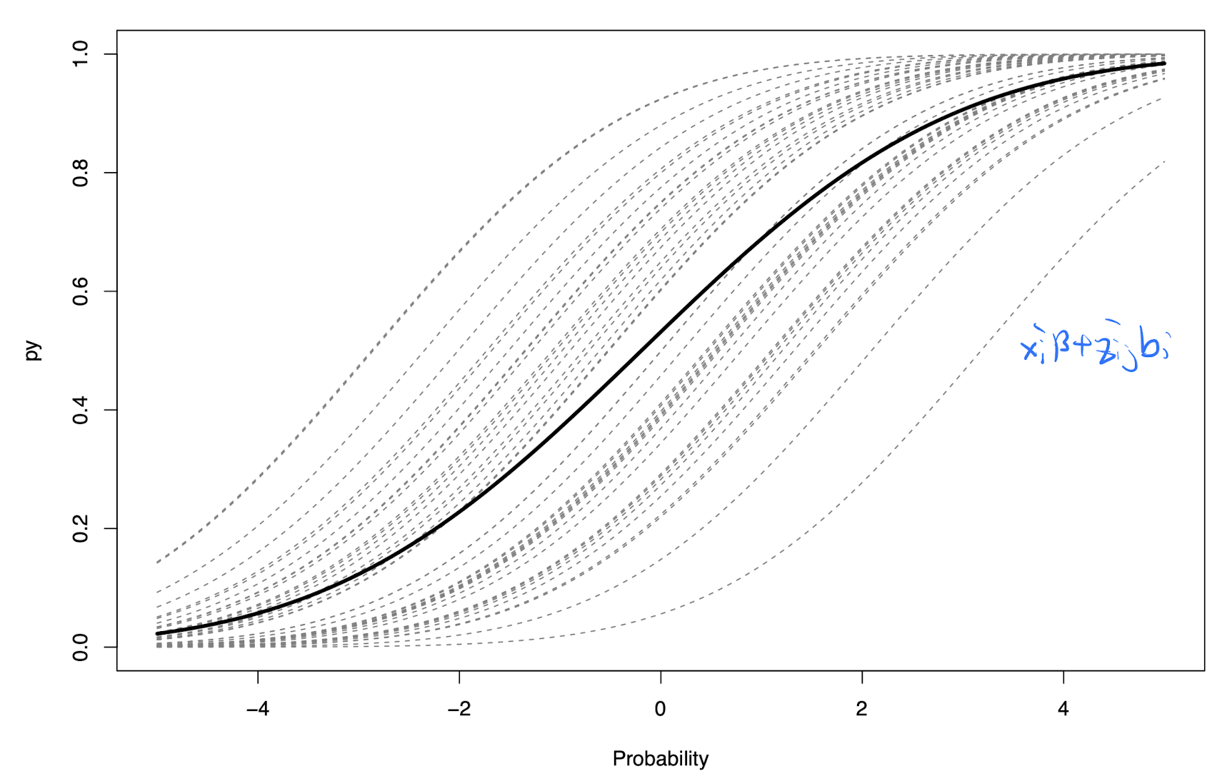

Consider \(Y_{ij} \sim Bernoulli(p_{ij})\), with \(\log \left( \frac{p_{ij}}{1 - p_{ij}} \right) = x_{ij}'\beta + b_i\), and \(b_i \sim_{iid} N(0, \sigma^2)\)

The marginal expectation is

\[E(Y) = E\{E(Y \mid b)\} = E \left[ \frac{\exp\{X\beta + b\}}{1 + \exp\{X\beta + b\}} \right] \approx \frac{\exp\{X\gamma\}}{1 + \exp\{X\gamma\}}\]

where \(\gamma = \frac{\beta}{\sqrt{c^2\sigma^2 + 1}}\), and \(c = 16\sqrt{3}/(15\pi)\)

Notes:

Further complications arise if \(\log \left( \frac{p_{ij}}{1 - p_{ij}} \right) = x_{ij}'\beta + z_{ij}'b_i\), in which case

\[\gamma \approx \beta |c^2 D(\alpha)ZZ' + I|^{-(q+1)/2}\]

Note: \(|c^2 D(\alpha)ZZ' + I|\) involves a diagonal matrix.

6.17 Numerical Note (Numerical Integration)

\[\mathcal{L}(\beta, \alpha) = \prod_{i=1}^n \int p(y_i \mid b_i) p(b_i) \, db_i\]

Numerical integration is at the heart of many statistical problems – Quadrature techniques:

Newton-Cotes quadrature
Trapezoidal quadrature
Gaussian quadrature
Adaptive quadrature

Asymptotic approximations:

Laplace approximations
INLA

Monte Carlo Methods

6.18 Newton-Cotes quadrature

Consider estimating

\[I = \int_a^b f(x) \, dx\]

Partition \([a, b]\) into \(n\) subintervals \([x_i, x_{i+1}]\), \(i = 0, 1, \dots, n-1\), with \(x_0 = a\) and \(x_n = b\):

\[\hat{I}_n = \sum_{i=0}^{n-1} f(x_i)(x_{i+1} - x_i)\]

Notes: * In undergrad, used Riemann integrals. * \(\lim_{n \to \infty} \hat{I}_n \to I\).

6.19 Trapezoidal Quadrature

Using local linear interpolations:

\[\hat{I}_n = \sum_{i=0}^{n-1} \frac{x_{i+1} - x_i}{2} \{f(x_i) + f(x_{i+1})\}\]

More generally, we could use local polynomial interpolations.

6.20 Gaussian Quadrature

Choose \((x_0, x_1, \ldots, x_n)\) evaluation points and a local polynomial of degree \(m\) to provide exact interpolation to \(f(x)\).

We often work with standardized orthogonal polynomials.

The Gaussian quadrature solution involves:

(i) \(I = \displaystyle\int_a^b f(x)\, dx = \int_a^b g(x)\, w(x)\, dx\), with \(w(x) > 0,\ \forall\, x\)

(ii) \(\hat{I}_n = \displaystyle\sum_{i=1}^n A_i f(x_i)\)

6.21 Multidimensional Integration

The integral:

\[I = \int_a^b \int_c^d f(x, y)\, dx\, dy\]

requires recursive estimation:

(i) \(\hat{g}_n(y) \approx \displaystyle\int_c^d f(x, y)\, dx\)

(ii) \(\hat{I}_n \approx \displaystyle\int_a^b \hat{g}(y)\, dx\)

In general, a \(p\)-dimensional integral requires \(n^p\) evaluations of \(f(\cdot)\).

In high dimensions, asymptotic expansions or Monte Carlo methods tend to scale more gracefully.

6.22 Laplace Approximations for Multiple Integrals

Let \(f : \mathbb{R}^p \to \mathbb{R}\), and write \(f(x) = \exp\{n h(x)\}\).

Use a Taylor expansion around \(\hat{x}\):

\[h(x) \approx h(\hat{x}) + (x - \hat{x})^\top h'(x)\big|_{\hat{x}} + \frac{1}{2}(x - \hat{x})^\top H(x)\big|_{\hat{x}} (x - \hat{x})\]

Leading to

\[\int_A \exp\{n h(x)\}\, dx \approx e^{h(\hat{x})} (2\pi)^{p/2} |H(\hat{x})|^{-1/2} \int_A \mathcal{N}\!\left(\hat{x},\, -H(\hat{x})^{-1}\right) dx\]

Important methodological extensions consider Nested Laplace Approximations.

6.23 Empirical Bayes Estimation of Random Effects

Given \(\hat{\beta}\) and \(\hat{\alpha}\), empirical Bayes estimates of the random effects \(b_i\) are obtained maximizing the posterior distribution

\[p(b_i \mid Y_i, \hat{\beta}, \hat{\alpha}) \propto p(Y_i \mid b_i, \hat{\beta}, \hat{\alpha}) p(b_i \mid D(\hat{\alpha}))\]

So that

\[\hat{b}_i = \text{Arg} \max_{b_i} p(b_i \mid Y_i, \hat{\beta}, \hat{\alpha})\]

In contrast to linear mixed models, \(\hat{b}_i\) is not available in closed form and needs to usually be derived numerically.