7  Marginal Models For Longitudinal Data

7.1 Motivation

• In some cases interest centers on population-level (marginal) quantities
• Mixed and Hierarchical models require correct specification of sampling distributions to achieve consistency
• Combine Quasi-Likelihood and Sandwich estimation to work with empirical summaries, rather than model-based assumptions

7.2 Back to LMM

In the linear case, we specify a conditional sampling distribution

\[Y_i \mid b_i \sim N(X_i\beta + Z_ib_i, \sigma^2_\epsilon I_{n_i}), \quad i = 1, 2, \ldots, m\]

Together with random effects

\[b_i \sim N_q(0, D(\alpha))\]

Leading to the marginal likelihood

\[Y_i \sim N(X_i\beta, V_i(\alpha, \sigma^2_\epsilon))\]

where

\[V_i(\alpha, \sigma^2_\epsilon) = Z_iD(\alpha)Z_i' + \sigma^2_\epsilon I_{n_i}\]

7.3 Likelihood Inference for LMM

Consider \(\alpha, \sigma^2_\epsilon\) known

The marginal likelihood estimate of \(\beta\) is obtained setting the score function to zero, i.e. solving the system of estimating functions

\[\frac{\partial \ell_m}{\partial \beta} = \sum_i X_i' V_i(\alpha, \sigma^2_\epsilon)^{-1}(Y_i - X_i\beta) = 0\]

Leading to

\[\hat{\beta} = \left(\sum_i X_i' V_i^{-1} X_i\right)^{-1} \left(\sum_i X_i' V_i^{-1} Y_i\right)\]

Relying on the assumption of Normality

\[\hat{\beta} \sim N\left[\beta, \left(\sum_i X_i' V_i^{-1} X_i\right)^{-1}\right]\]

Relying on asymptotic approximations

\[\text{Var}(\hat{\beta}) \approx -E\left(\frac{\partial^2 \ell_m}{\partial \beta \partial \beta'}\right) = \left(\sum_i X_i' V_i^{-1} X_i\right)^{-1}\]

7.4 LMM and Estimating Equations

Consider the linear Estimating Equations

\[G_m(\beta) = \sum_i X_i' V_i^{-1}(Y_i - X_i\beta) = \frac{1}{m} \sum_i G_i(\beta, Y_i) := 0\]

Assuming \(E(Y_i) = X_i\beta\) (i.e. assuming we have the correct model for \(Y_i\))

\[E[G_i(\beta, Y_i)] = E[X_i' V_i^{-1}(Y_i - X_i\hat{\beta})] = X_i' V_i^{-1} E[(Y_i - X_i\beta)] = 0\]

For simplicity consider \(\beta \in \mathbb{R}\). Assume \(\hat{\beta} \overset{p}{\to} \beta\) A Taylor approximation to \(G_m(\beta)\) around \(\beta\) (true value) gives

\[0 = G_m(\hat{\beta}) = G_m(\beta) + (\hat{\beta} - \beta)\frac{dG_m}{d\beta}\bigg|_{\beta} + \frac{1}{2}(\hat{\beta} - \beta)^2 \frac{d^2G_m}{d\beta d\beta'}\bigg|_{\tilde{\beta}}\]

where \(\tilde{\beta}\) is a value between \(\hat{\beta}\) and \(\beta\)

Leading to

\[(\hat{\beta} - \beta) = -G_m(\beta) \left/ \frac{dG_m}{d\beta}\bigg|_{\beta} + \frac{1}{2}(\hat{\beta} - \beta)\frac{d^2G_m}{d\beta d\beta'}\bigg|_{\tilde{\beta}}\right.\]

We now determine the asymptotic distribution of the right-hand side

7.5 Limiting Distributions

Going back to \(\beta \in \mathbb{R}^p\), we have

\[B_m(\beta)^{-1/2} G_m(\beta) \to_d N(0, I_m)\]

where

\[B_m(\beta) = \text{Var}(G_m(\beta)) = E[G_m(\beta)G_m(\beta)']\]

The first term in the denominator

\[\frac{\partial G_m}{\partial \beta}\bigg|_{\beta} = \frac{1}{m}\sum_i \frac{\partial}{\partial \beta} G_i(\beta, Y_i)\bigg|_{\beta} \to_p E\left(\frac{\partial}{\partial \beta} G_m(\beta)\right) = A_m(\beta)\]

Applications of WLLN + Slutsky leads to

\[[A_m^{-1} B_m (A_m')^{-1}]^{-1/2} (\hat{\beta} - \beta) \to_d N(0, I_p)\]

We have

\[[A_m^{-1} B_m (A_m')^{-1}]^{-1/2} (\hat{\beta} - \beta) \to_d N(0, I_p)\]

If we are willing to rely on the Likelihood, then

\[G_m = \frac{\partial}{\partial \beta} \ell_m(\beta) = S_m(\beta), \quad \text{and} \quad B_m = -A_m\]

because

\[I_m(\beta) = -E\left(\frac{\partial S_m(\beta)}{\partial \beta'}\right) = E[S_m(\beta)S_m(\beta)']\]

Therefore

\[A_m^{-1} B_m (A_m')^{-1} = A_m^{-1}, \quad \text{with} \quad A_m = \left(\sum_i X_i' V_i^{-1} X_i\right)\]

7.6 Empirical/Robust Estimation

Instead of relying on theoretical expectations, define

\[\hat{A}_m = \frac{1}{m}\sum_i \frac{d}{d\beta} G_i(\hat{\beta}, Y_i) = -\sum_i X_i' V_i^{-1} X_i\]

and

\[\hat{B}_m = \frac{1}{m} G_m(\hat{\beta})G_m(\hat{\beta})' = \sum_i [X_i' V_i^{-1}(Y_i - X_i\beta)(Y_i - X_i\beta)'V_i^{-1}X_i]\]

Leading to the sandwich estimator

\[V(\hat{\beta}) = \left(\sum_i X_i' V_i^{-1} X_i\right)^{-1} \left(\sum_i X_i' V_i^{-1}(Y_i - X_i\beta)(Y_i - X_i\beta)'V_i^{-1}X_i\right) \left(\sum_i X_i' V_i^{-1} X_i\right)^{-1}\]

Note: We have empircal covariance of the estimator in the center, it is a robust way of estimating the covariance. It uses empirical observations to make robust estimators (or something like that).

Example 7.1 (Pig Diet)  

Pig Diet

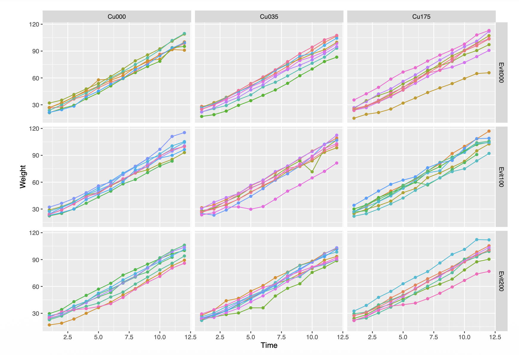
fit1 = lmer(Weight ~ Evit*Time + (1|Pig), data=dietox)
mf <- formula(Weight ~ Evit*Time)
fit2 <- geeglm(mf, data=dietox, id=Pig, family=gaussian("identity"),
corstr="exchangeable")

Here, we assume exchangeability in our covariance structure.

	fit1	fit2
Coefficients (Std. Error)
(Intercept)	15.3089 (1.3828)	15.3089 (1.065)
EvitEvit100	1.2702 (1.9354)	1.2702 (1.361)
EvitEvit200	-0.0307 (1.9162)	-0.0307 (1.393)
Time	6.9649 (0.0584)	6.9649 (0.138)
EvitEvit100:Time	0.1172 (0.0821)	0.1172 (0.193)
EvitEvit200:Time	-0.1756 (0.0811)	-0.1756 (0.192)

7.7 Estimating Functions

Definition 7.1 (Estimating Function) Let \(Y_i \sim_{iid} F(\theta)\), \(i = 1, 2, \ldots, n\)

An estimating function

\[G_n(\theta) = \frac{1}{n}\sum_i G(\theta, Y_i)\]

is a function of the same dimension as \(\theta\), for which

\[E[G_n(\theta)] = 0\]

Definition 7.2 (Estimating Equation) The corresponding estimating equation defines the estimator \(\hat{\theta}_n\) as follows:

\[G_n(\hat{\theta}_n) = \frac{1}{n}\sum_i G(\hat{\theta}_n, Y_i) = 0\]

7.8 Estimating Functions Asymptotics

\(G_n(\theta)\) is a sum of independent random variables \(\ldots\) WLLN - CLT \(\ldots\)

Proposition 7.1 (Estimating Functions Asymptotics) Let \(\hat{\theta}_n\) be a solution to the estimating function, s.t. \(G_n(\hat{\theta}_n) = 0\), then:

(1) \(\hat{\theta}_n \to_p \theta\)

(2) \(\sqrt{n}(\hat{\theta}_n - \theta) \to_d N\left(0, A^{-1}B(A')^{-1}\right)\)

where

\[A = A(\theta) = E\left(\frac{\partial}{\partial \theta'} G(\theta, Y)\right)\]

and

\[B = B(\theta) = E[G(\theta, Y)G(\theta, Y)'] = \text{Var}[G(\theta, Y)]\]

Note: As long as the epxectation of \(G_n(\hat{\theta_n}) = 0\), it satisifes this above properties.

7.9 General - Non iid Case

In most regression setting \(Y_i \perp Y_j\), but their sampling distributions are not assumed identical

(1) \(\hat{\theta}_n \to_p \theta\)

(2) \(\left(A_n^{-1} B_n (A_n')^{-1}\right)^{-1/2} (\hat{\theta}_n - \theta) \to_d N[0, I_k]\)

where

\[A_n(\theta) = E\left(\frac{\partial}{\partial \theta'} G_n(\theta)\right)\]

and

\[B_n(\theta) = E[G_n(\theta)G_n(\theta)'] = \text{Var}[G_n(\theta)]\]

7.10 MLE as a Special Case

If we are willing to assume a specific sampling model \(p(Y_i \mid \theta)\), \(\theta \in \mathbb{R}^k\). The log-likelihood is

\[\ell(\theta) = \sum \log p(Y_i \mid \theta)\]

with score function

\[S(\theta) = \frac{\partial \ell(\theta)}{\partial \theta} = \left(\frac{\partial \ell(\theta)}{\partial \theta_1}, \ldots, \frac{\partial \ell(\theta)}{\partial \theta_k}\right)' = [S_1(\theta), \ldots, S_k(\theta)]'\]

with \(E(S(\theta)) = 0\) (under regularity conditions).

Viewing the score as an estimating function

\[G_n(\theta) = \frac{1}{n} S(\theta) = \frac{1}{n}\sum_i \frac{\partial}{\partial \theta} \log p(Y_i \mid \theta)\]

Viewing the score as an estimating function

\[G_n(\theta) = \frac{1}{n} S(\theta) = \frac{1}{n}\sum_i \frac{\partial}{\partial \theta} \log p(Y_i \mid \theta)\]

\(A(\theta) = E\left(\frac{\partial}{\partial \theta'} G(\theta, Y)\right) = E\left[\frac{\partial^2}{\partial \theta \partial \theta'} \log p(Y \mid \theta)\right]\)

\(B(\theta) = E[G(\theta, Y)G(\theta, Y)'] = E\left[\frac{\partial}{\partial \theta} \log p(Y \mid \theta) \left(\frac{\partial}{\partial \theta} \log p(Y \mid \theta)\right)'\right]\)

The MLE \(\hat{\theta}_n\), solving \(G_n(\hat{\theta}_n) = 0\), is asymptotically Normal

\[\hat{\theta}_n \approx_d N\left(\theta, (A^{-1}B(A')^{-1})\right) \equiv N\left(\theta, I(\theta)^{-1}\right), \quad \text{as } n \to \infty\]

7.11 Quasi Likelihood

Quasi Likelihood avoids reliance on sampling model/distribution

Rather than specifying a sampling model, only specify the first two moments

\[E(Y \mid \beta) = \mu(\beta)\]

\[\text{Var}(Y \mid \beta, \alpha) = V[\alpha, \mu(\beta)], \quad \alpha > 0\]

Notice that variance struccure may also be indexed by \(\mu(\beta)\), i.e. it involves \(\beta\)

QL estimating functions are often based on the GLS

\[[Y - \mu(\beta)]'V^{-1}[Y - \mu(\beta)]\]

Should remind you of score for the GLM, at least the veneral structure

Treating \(V\) as a nuisance and differentiating wrt. \(\beta\) leads to

\[G(\hat{\beta}) = D(\hat{\beta})'V(\alpha, \hat{\beta})^{-1}[Y - \mu(\hat{\beta})] := 0\]

with \(D(\beta) : n \times p\), s.t. \(D_{ij} = \frac{\partial \mu_i(\beta)}{\partial \beta_j}\)

We have

\[(D'V^{-1}D)^{1/2}(\hat{\beta}_n - \beta) \to_d N(0, \alpha I_p)\]

In practice a consistent estimator of \(\alpha\) is plugged in. E.g.:

\[\hat{\alpha} = (Y - \hat{\mu})'V^{-1}(Y - \mu)/(n - p)\]

• Construction of estimating functions is only based on the first two moments
• The resulting sampling model may not correspond to a specific distribution
• No probabilistic prediction is usually warranted

• 7.12 Consistency depends only on specifying correctly the mean structure

  If we get variance wrong, doesn’t matter. Asymptotically, estimator will converge to the truth.

• Asymptotically appropriate standard errors depend on the correct specification of the mean/variance relationship
• QL estimators are likely to be consistent in a wider range of circumstances than ML estimators

Example 7.2 (QL Estimating Function) Consider data from a counting process, s.t.

\[E(Y_i) = \theta, \quad V(Y_i) = \alpha\theta; \quad \alpha > 0\]

The GLS-QL estimating functions take the form

\[\frac{1}{n}\sum_i \frac{1}{\alpha\theta}(Y_i - \theta) := 0\]

Leading to

\[\hat{\theta}_n = \bar{Y}_n\]

If \(\hat{\alpha} = \frac{1}{n-1}\sum(Y_i - \hat{\theta})^2/\hat{\theta} = S^2/\bar{Y}\)

The asymptotic variance of \(\hat{\theta}\) is \(\widehat{\text{Var}}(\hat{\theta}) = S^2/n\)

7.13 Sandwich Estimation

Consider the estimating function \(G_n(\theta) = \frac{1}{n}\sum_{i=1}^n G(\theta, Y_i)\). We have that \(\text{Cov}(\hat{\theta}) = A_n^{-1} B_n (A_n')^{-1}\), with

\[A_n(\theta) = E\left(\frac{\partial}{\partial \theta} G_n(\theta, Y)\right)\]

\[B_n(\theta) = E[G_n(\theta, Y) G_n(\theta, Y)']\]

For these expectations to provide asymptotically adequate variance estimates, they need to be evaluated under the true model. The idea behind sandwich estimation is to evaluate these expectations empirically.

Empirical estimation of variance components:

\[\hat{A}_n = \frac{1}{n}\sum_i \frac{\partial}{\partial \theta} G(\hat{\theta}, Y_i)\]

\[\hat{B}_n = \frac{1}{n}\sum_i G(\hat{\theta}, Y_i)G(\hat{\theta}, Y_i)'\]

By WLLN \(\hat{A}_n \to_p A_n\), and \(\hat{B}_n \to_p B_n\), where

\[\text{Var}(\hat{\theta}) = \hat{A}_n^{-1} B_n (\hat{A}_n')^{-1}\]

is a consistent estimator of the variance.

Some properties of the sandwich estimation:

• Sandwich estimation provides consistent estimation of the variance under very broad circumstances

• Possibly unstable in small samples

• If the mean/variance relationship is tight, model-based estimation is more efficient

7.14 QL + Sandwich

Consider a simple setting where we only assume

\[E(Y_i) = \mu_i(\beta)\]

\[V(Y_i) = \alpha V(\mu_i)\]

\[\text{Cov}(Y_i, Y_j) = 0\]

The quasi score is

\[G(\hat{\beta}) = \sum_i D_i V_i^{-1}\left(Y_i - \mu_i(\hat{\beta})\right) := 0\]

Leading to an estimator of \(\beta\) with variance

\[\text{Var}(\hat{\beta}) = \left(D'V^{-1}D\right)^{-1} \left(D'V^{-1}\text{Var}(Y)V^{-1}D\right) \left(D'V^{-1}D\right)^{-1}\]

A simple consistent estimator of \(\text{Var}(Y)\) is, for example

\[\text{diag}(RR') = \text{diag}(Y_i - \hat{\mu}_i)(Y_i - \hat{\mu}_i)'\]

Example 7.3 (Sandwich Estimator) Consider data from a counting process, s.t.

\[E(Y_i) = \theta, \quad V(Y_i) = \alpha\theta; \quad \alpha > 0\]

Verify

\[\hat{A} = -\frac{1}{n}\sum_i \frac{Y_i}{\hat{\theta}^2} = -\frac{1}{\bar{Y}}\]

\[\hat{B} = \frac{1}{n}\sum_i \frac{(Y_i - \hat{\theta})^2}{\hat{\theta}^2} = \frac{(n-1)S^2}{n\hat{\theta}^2}\]

leading to the sandwich estimator of the variance

\[\widehat{\text{Var}}(\hat{\theta}) = \frac{S^2}{n} \cdot \frac{(n-1)}{n}\]

7.15 GEE for Longitudinal Linear Models

Consider longitudinal data \(Y_i = (Y_{i1}, \ldots, Y_{im_i})'\), \(i = 1, \ldots, n\). Assume \(E(Y_i) = X_i\beta\).

Consider a working covariance \(\text{Cov}(Y_i) = W_i(\alpha, \beta)\)

For known \(W_i\), a GLS estimating function is obtained from the weighted LS

\[\sum_i (Y_i - X_i\beta)'W_i^{-1}(Y_i - X_i\beta)\]

Leading to the estimating equation

\[\sum_i X_i' W_i^{-1}(Y_i - X\hat{\beta}) := 0\]

This yields

\[\hat{\beta} = \left(\sum_i X_i' W_i^{-1} X_i\right)^{-1} \left(\sum_i X_i' W_i^{-1} Y_i\right)\]

7.16 Properties of \(\hat{\beta}\)

\[E(\hat{\beta}) = \beta\]

\[\hat{\beta} \to_p \beta, \quad \text{independently of } W_i\]

\[\text{Var}(\hat{\beta}) = \left(\sum_i X_i' W_i^{-1} X_i\right)^{-1} \left(\sum_i X_i' W_i^{-1} \text{Cov}(Y_i) W_i^{-1} X_i\right) \left(\sum_i X_i' W_i^{-1} X_i\right)^{-1}\]

If we are willing to maintain our assumption \(\text{Cov}(Y_i) = W_i\), then

\[\text{Var}(\hat{\beta}) = \left(\sum_i X_i' W_i^{-1} X_i\right)^{-1}\]

7.17 GEE Algorithm

• Clearly \(W_i(\alpha, \beta)\) is usually unknown
• Depending on the form of \(W_i\), estimators of \(\beta\) may have to derived numerically
• Substantial simplifications arise if \(W_i = W_i(\alpha)\)
• In this setting a stable estimator \(\hat{\alpha}\) of \(\alpha\), leads to \(\hat{W}_i = W_i(\hat{\alpha})\)
• An empirical estimator of \(\text{Cov}(Y_i)\) is obtained as

\[\hat{\Sigma}_i = \widehat{\text{Cov}}(Y_i) = (Y_i - X_i\hat{\beta})'(Y_i - X_i\hat{\beta})\]

so that

\[\text{Var}(\hat{\beta}) = \left(\sum_i X_i' \hat{W}_i^{-1} X_i\right)^{-1} \left(\sum_i X_i' \hat{W}_i^{-1} \hat{\Sigma}_i \hat{W}_i^{-1} X_i\right) \left(\sum_i X_i' \hat{W}_i^{-1} X_i\right)^{-1}\]

7.18 Variance Parameters

• Formally a second estimating equation may be introduced for the estimation of the variance parameters \(\alpha\)

\[G_1(\beta, \alpha) = \sum_i X_i' W_i^{-1}(Y_i - X_i\beta)\]

\[G_2(\beta, \alpha) = \sum_i E_i' H_i^{-1}(T_i - \Sigma_i(\alpha))\]

• See Wakefield for details

7.19 GEE Summary

(1) Specify a mean model \(E(Y_i) = X_i\beta\)

(2) Specify a working covariance \(\text{Var}(Y_i) = W_i(\alpha)\)

(3) Construct and estimating function from (1) and (2) and use sandwich estimation of the variance

• A consistent estimator of \(\beta\) only relies on the correct specification of the first moment
• Specifying \(W_i\) incurs the usual efficiency/robustness trade off
• Usually no probabilistic prediction is warranted
• Inference relies on asymptotics
• Sandwich SE may be unstable for small samples

7.20 GEE for Longitudinal GLM

Consider

\[p(y_{ij}) = \exp\{[y_{ij}\theta_{ij} - b(\theta_{ij})]/a(\alpha) - c(y_{ij}, \alpha)\}\]

\(E(Y_{ij}) = \mu_{ij}\), and \(g(\cdot)\) being a link function

Assume

\[g(\mu_{ij}) = x_{ij}'\beta\]

\[\text{Var}(Y_i) = W_i\]

Define \(D_i = \frac{\partial \mu_i}{\partial \beta}\), and construct the estimating equation

\[G(\beta, \hat{\alpha}) = \sum_i D_i' W_i^{-1}\left(Y_i - \mu_i(\hat{\beta})\right) := 0\]

7.21 Properties of \(\hat{\beta}\)

(1)

\[V_\beta = \left(\sum_i D_i' W_i^{-1} D_i\right)^{-1} \left(\sum_i D_i' W_i^{-1} \text{Cov}(Y_i) W_i^{-1} D_i\right) \left(\sum_i D_i' W_i^{-1} D_i\right)^{-1}\]

(2)

\[V_\beta^{-1/2}(\hat{\beta}_n - \beta) \to_d N(0, I_p)\]

7.22 Summary

• GEE appealing as it only requires correct specification of the mean for consistent estimation of \(\beta\)
• In GLM we retain the marginal interpretation of regression coefficients
• Asymptotic reliability relies on large \(n\)
• Asymptotic efficiency relies on \(W_i\)
• Published work is conflictual on recommendations for \(W_i\)
• Extreme care is needed when missing data are not CAR
• Recent work introduced doubly robust estimation to deal with missingness
• No probabilistic prediction is warranted
• No subject-level inference is warranted