5  Linear Mixed Effects Models (LMEM)

5.1 Linear Mixed Effects Models

If we can operate under Gaussian sampling, let \(Y_i = (Y_{i1}, \dots, Y_{im})'\).

A Linear Mixed Effects Model assumes:

\[Y_i = X_i \beta + Z_i b_i + \epsilon_i\]

with

1. \(\epsilon_i : m \times 1 \sim N\{0,\ E(\alpha)\}\)

2. \(b_i : k \times 1 \sim N\{0,\ D(\alpha)\}\)

3. \(\epsilon_i \perp b_i, \quad b_i \perp b_j\)

5.2 LMM Marginal Moments

The model:

\[Y_i = X_i \beta + Z_i b_i + \epsilon_i, \qquad b_i \sim N(0,\ D(\alpha));\]

yields closed form marginal moments:

\[\circ \quad E(Y_i) = X_i \beta\]

\[\circ \quad \text{Cov}(Y_i) = Z_i D(\alpha) Z_i' + E(\alpha) = V_i(\alpha)\]

\[\circ \quad \text{Cov}(Y_i, Y_j) = 0, \quad \text{for any } i \neq j\]

5.3 LMM Fixed Effects

\[p(Y \mid \beta,\ \alpha) = \prod_i \int p(Y_i \mid \beta,\ \alpha,\ b_i)\, dp(b_i \mid \alpha)\]

• Using the fact that convolutions of Normals are Normal

\[Y_i \mid \beta, \alpha \sim N(X_i \beta,\ V_i(\alpha))\]

Leading to the marginal log-likelihood

\[\ell(\beta,\ \alpha) = -\frac{1}{2} \sum_i \log |V_i(\alpha)| - \frac{1}{2} \sum_i (y_i - X_i \beta)' V_i(\alpha)^{-1} (y_i - X_i \beta)\]

5.4 (LMM) Inference for Fixed Effects

The marginal log-likelihood is

\[\ell(\beta,\ \alpha) = -\frac{1}{2} \sum_i \log |V_i(\alpha)| - \frac{1}{2} \sum_i (y_i - X_i \beta)' V_i(\alpha)^{-1} (y_i - X_i \beta)\]

The corresponding score equations for \(\beta\) are:

\[\frac{\partial \ell(\cdot)}{\partial \beta} = \sum_i X_i' V_i(\alpha)^{-1}(y_i - X_i \beta) := 0\]

Produce the familiar GLS estimator of \(\beta\)

\[\hat{\beta}(\alpha) = \left\{ \sum_i X_i' V_i(\alpha)^{-1} X_i \right\}^{-1} \left\{ \sum_i X_i' V_i(\alpha)^{-1} Y_i \right\}\]

5.5 ML Asymptotics

The expected Information is block diagonal

\[I(\beta,\ \alpha) = \begin{bmatrix} I_{\beta\beta} & 0 \\ 0 & I_{\alpha\alpha} \end{bmatrix}\]

with

\[I_{\beta\beta} = -E\left[\frac{\partial^2 \ell(\beta,\ \alpha)}{\partial\beta\, \partial\beta'}\right] = \sum_i X_i' V_i(\alpha)^{-1} X_i\]

For any consistent estimator \(\hat{\alpha}\) of \(\alpha\)

\[\left(\sum_i X_i' V_i(\hat{\alpha})^{-1} X_i\right)^{1/2} (\hat{\beta}_n - \beta) \longrightarrow_d N(0,\ I_q)\]

• Testing based on LRT follows standard theory

• Several corrections aimed at improving finite sample operating characteristics

5.6 Where Are We Going

• Inference for variance components via ML
• Inference for variance components via REML
• Inference for random effects
• Bayesian Inference

5.7 Inference for Variance Components Via Maximum Likelihood (ML)

Because \(\hat{\beta}(\alpha)\) is available in closed form via GLS, the MLE \(\hat{\alpha}\) is most conveniently obtained via numerical maximization of the profile log-likelihood

\[\ell_p(\alpha) = -\frac{1}{2} \sum_i \log |V_i(\alpha)| - \frac{1}{2} \sum_i \{y_i - X_i\hat{\beta}(\alpha)\}' V_i(\alpha)^{-1} \{y_i - X_i\hat{\beta}(\alpha)\}\]

Standard Likelihood theory applies, with:

\[I_{\alpha\alpha}^{1/2}(\hat{\alpha}_n - \alpha) \longrightarrow_d N(0,\ I_r)\]

We note that \(E[Y_i|b_i] = X_i\beta + b_i + \epsilon_i\) where \(b_i \sim \mathcal{N}(0, \sigma^2_b)\) and \(H_0: \sigma^2_b = 0\).

Note on LRT involving \(\alpha\): be careful about testing variance since the test is on the boundary of the parameter space.

5.8 Restricted Maximum Likelihood

5.8.1 Inference for Variance Components Based on REML

• ML estimates of \(\alpha\) are biased in finite samples
• Alternative inference about \(\alpha\) is often based on Restricted (or Residual) Maximum Likelihood (REML) estimators
• REML provides a way to correct for the fact that the mean structure is unknown and needs to be estimated
• Intuitively one could proceed with data constructed from the distribution of the residuals \(Y - X\hat{\beta}\)

The idea is we want to remove any nuisance parameters to focus soley on estimating the parameter of interest.

5.8.2 Marginal Likelihood Without Priors

In the presence of nuisance parameters, different versions of the likelihood have been developed to yield estimators with improved finite sample characteristics

Marginal Likelihood

• Let \(S_1\), \(S_2\) be minimal sufficient statistics for \(\theta = (\lambda, \phi)\), and \(A\) be ancillary. Suppose we can write

\[p(y \mid \lambda,\ \phi) \propto p(a)\, p(s_1 \mid a,\ \lambda)\, p(s_2 \mid s_1,\ a,\ \lambda,\ \phi)\]

If \(\phi\) is a nuisance parameter, inference for \(\lambda\) may be based on the marginal likelihood

\[p(s_1 \mid a,\ \lambda)\]

Example 5.1 (Linear Regression) Let \(Y \sim N(X\beta,\ H(\theta))\). Consider data transformations \(U = f(Y)\) which do not depend on \(\beta\). A typical candidate consists of error contrasts \(a'Y\), based on vectors orthogonal to \(X\), s.t. \(a'X = 0\)

We can show that there exist only \((n - k)\) such vectors s.t. \(A'X = 0\), with a good candidate being \(I_n - X(X'X)^{-1}X'\). The contrast vector \(U = A'Y\) does not depend on \(\beta\), as

\[A'Y = A'(X\beta + \epsilon) = A'\epsilon \sim N(0,\ A'H(\theta)A)\]

Estimation of variance components \(\theta\) can be based on the restricted likelihood

\[L(\theta;\ u) = L(\theta;\ A'Y)\]

In short, what we’re trying to do is eliminate nuisance parameters (in this case, \(\beta\)) to estimate only our parameter of interest. We do this by using contrasts

5.8.3 Bayesian Interpretation of REML (Linear Regression)

Assume \(Y \sim N(X\beta,\ \sigma^2 I_n)\). An alternative way of deriving REML estimators is to introduce a prior on \(\beta\), s.t. \(p(\beta) \propto c\) and calculate the marginal likelihood as

\[p(y \mid \sigma^2) = \int p(y \mid \beta,\ \sigma^2)\, p(\beta)\, d\beta\]

We have

\[p(y \mid \sigma^2) \propto \frac{1}{\sigma^{n-k}} \exp\left\{-\frac{1}{2\sigma^2}(y - X\hat{\beta})'(y - X\hat{\beta})\right\}\]

producing

\[\hat{\sigma}^2_{\text{REML}} = \frac{RSS}{n - k}\]

5.8.4 REML for LMEM

Assume \(p(\beta) \propto c\) (a constant). The marginal likelihood for the LMEM is:

\[p(y \mid \alpha) \propto \prod_i |V_i(\alpha)|^{-1/2} \int \exp\left\{-\frac{1}{2}(y_i - X_i\beta)' V_i(\alpha)^{-1}(y_i - X_i\beta)\right\} d\beta\]

\[p(y \mid \alpha) \propto \prod_i |V_i(\alpha)|^{-1/2} \int \exp\left\{-\frac{1}{2}(y_i - X_i\beta)' V_i(\alpha)^{-1}(y_i - X_i\beta)\right\} d\beta\]

Expanding \((y_i - X_i\beta) = (y_i - X_i\hat{\beta}) + (X_i\hat{\beta} - X_i\beta)\):

\[\exp\left\{-\frac{1}{2}\left[(y_i - X_i\hat{\beta}) + (X_i\hat{\beta} - X_i\beta)\right]' V_i(\alpha)^{-1}(\cdots)\right\}\]

\[\leadsto\ \exp\left\{-\frac{1}{2}\,RSS\right\} \cdot \underbrace{ \exp\left\{-\frac{1}{2}(\beta - \hat{\beta})' \underbrace{X_i' V_i(\alpha)^{-1} X_i}_{\mathcal{I}} (\beta - \hat{\beta}_i)\right\} }_{\text{kernel of multivariate Gaussian distribution}}\]

Restricted Log-Likelihood

\[\ell_R(\alpha) = -\frac{1}{2}\sum_i \log|V_i(\alpha)| - \frac{1}{2}\sum_i \log|X_i' V_i(\alpha)^{-1} X_i| - \sum_i \frac{1}{2}\{y_i - X_i\hat{\beta}(\alpha)\}' V_i(\alpha)^{-1}\{y_i - X_i\hat{\beta}(\alpha)\}\]

To be compared with the profile log-likelihood:

\[\ell_p(\alpha) = -\frac{1}{2} \sum_i \log |V_i(\alpha)| - \frac{1}{2} \sum_i \{y_i - X_i\hat{\beta}(\alpha)\}' V_i(\alpha)^{-1} \{y_i - X_i\hat{\beta}(\alpha)\}\]

5.8.5 REML Comments

• Estimators based on \(\ell_R\) tend to still have finite sample bias, but they tend to perform better than ML, especially in small samples
• Asymptotics may still be based on \(I_R\)
• LRT on \(\alpha\), based on \(\ell_R\), still valid… with care…
• LRT on \(\beta\), based on \(\ell_R\), does not follow standard asymptotics

5.9 Random Effects

Example 5.2 (Dental Growth Study)  

Dental Growth Study

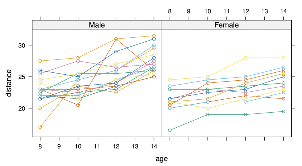
• Average growth within sex? [Marginal analysis]
• Boy/Girl-specific growth pattern? [Conditional analysis]

\[Y_i = \beta_0 + \beta_1\, Age + b_{0i} + b_{1i}\, Age + \epsilon_i, \qquad (b_{0i}, b_{1i}) \sim N(0, \Sigma).\]

\[E(Y_i \mid b_i) = X_i\beta + b_{i0} + b_{i1}\, t\]

\[\begin{bmatrix} b_{i0} \\ b_{i1} \end{bmatrix} \sim N(0,\ \Sigma)\]

Table 1: Dental Growth: Comparison of MLE and REML estimators

	ML	SE(ML)	T(ML)	REML	SE(R)	T(R)
(Intercept)	16.76	0.76	22.03	16.76	0.78	21.62
age	0.66	0.07	9.44	0.66	0.07	9.27

R Output:

# MLE -------------
s1$varcor

## Groups  Name        Std.Dev. Corr
## Subject (Intercept) 2.19408
##         age         0.21492  -0.581
## Residual            1.31005

# REML ------------
s2$varcor

## Groups  Name        Std.Dev. Corr
## Subject (Intercept) 2.32736
##         age         0.22645  -0.609
## Residual            1.31002

5.9.1 Inference for Random Effects

• Because \(b_i\) is a random variable (not an unknown constant), frequentist estimation yields a prediction problem
• Minimize the MSE, for any matrix \(A > 0\):

\[MSE(\tilde{b}) = E_y[E_b\{(\tilde{b} - b)'A(\tilde{b} - b)\}]\]

• We can show that \(\hat{b} = E(b \mid Y)\) (Robinson, 1991)

\[\begin{bmatrix} b_i \\ y_i \end{bmatrix} \sim N\left(\begin{bmatrix} 0 \\ X_i\beta \end{bmatrix},\ \begin{bmatrix} D(\alpha) & D(\alpha)Z_i' \\ Z_i D(\alpha) & V_i(\alpha) \end{bmatrix}\right)\]

Producing

\[\hat{b}_i = E(b_i \mid y_i, \beta, \alpha) = D(\alpha) Z_i' V_i(\alpha)^{-1}(y_i - X_i\beta)\]

\[\text{Var}(b_i \mid y_i, \beta, \alpha) = D(\alpha) - D(\alpha)Z_i' V_i(\alpha)^{-1} Z_i D(\alpha)\]

5.10 Empirical Bayes Estimation of Random Effects

\[p(b_i \mid Y) = \int f(b_i, \alpha, \beta \mid Y)\, d\beta\, d\alpha\]

with \(p(\beta) \propto c\) and \(p(\alpha) \propto \text{Id}^{-1}\).

\[E[b_i \mid Y, \alpha] = D(\alpha) Z_i' V_i(\alpha)^{-1}(y_i - X_i\hat{\beta}_{GLS})\]

\[\Rightarrow E(b_i \mid Y) = ?\]

\[\text{Var}(b_i \mid Y, \alpha) = \ldots\]

\[\text{Var}(b_i \mid Y) = ?\]

5.10.1 Bayesian Inference for LMEM

Classical LMEM:

\[Y_i = X_i\beta + Z_i b_i + \epsilon_i, \qquad b_i \sim_{iid} N(0, D) \perp \epsilon_i \sim_{iid} N(0,\ \sigma_\epsilon^2 I_{m_i}).\]

Hierarchical Model

(Stage One): Likelihood

\[p(y_i \mid \beta,\ b_i,\ \sigma_\epsilon^2), \quad i = 1, 2, \dots, m\]

(Stage Two): Random Effects Prior

\[p(b_i \mid D), \quad i = 1, 2, \dots, m\]

(Stage Three): Hyperprior

\[p(\beta,\ D,\ \sigma_\epsilon^2)\]

5.10.2 Hyperpriors

It is common to assume

\[p(\beta,\ D,\ \sigma_\epsilon^2) = p(D)\, p(\sigma_\epsilon^2)\, p(\beta \mid \sigma_\epsilon^2)\]

with

\[\sigma_\epsilon^2 \sim IG(a,\ b)\]

\[\beta \mid \sigma^2 \sim N\!\left(\beta_0,\ \frac{\sigma^2}{\delta}(X'X)^{-1}\right) \quad \leftarrow \text{Zellner}\]

\[D \sim IW_r(v,\ S) \quad \leftarrow \text{inverse Wishart}\]

Note: see Horsfield for alternative priors.

5.10.3 Bayesian Inference for LMEM

• Inference is based on the posterior distribution

\[p(\beta,\ b,\ D,\ \sigma_\epsilon^2 \mid Y)\]

• Simulation-based inference is often implemented via MCMC
• An efficient Gibbs sequence simulates iteratively from the following distributions:

1. \(p(\beta, b \mid Y, D, \sigma_\epsilon^2) = p(b \mid Y, \beta, D, \sigma_\epsilon^2)\, p(\beta \mid Y, D, \sigma_\epsilon^2)\)

2. \(p(\sigma_\epsilon^2 \mid Y, \beta, b)\)

3. \(p(D \mid Y, \beta, b, \sigma_\epsilon^2)\)

5.10.4 Hierarchical Centering for LMEM

• The efficiency of MCMC simulations can often be improved through re-parametrization
• (Gelfand, et al. 1995) suggest centering the model as follows

Assuming \(X_i \equiv Z_i\),

Stage 1: Likelihood

\[Y_i = X_i b_i + \epsilon_i, \qquad \epsilon_i \sim_{iid} N(0,\ \sigma_\epsilon^2 I_{m_i})\]

Stage 2: Subject-level prior

\[b_i \mid \beta \sim_{iid} N(\beta,\ D)\]

Stage 3: Hyperprior

\[p(\beta,\ D,\ \sigma_\epsilon^2)\]