8 Conditional Independence and Graphical Models
8.1 Motivation
8.2 Undirected Graphs
8.2.1 Some Basic Concepts (Undirected Graphs)
Definition 8.1 (Unhdirected Graphs Basic Concepts) Consider a random vector \(X = \{X_v ; v \in V\}\) together with a graph \(G = \{V, E\}\), whose nodes index components of \(X\).
- We interpret an edge \((v, w) \in E\) as a form of dependence between \(X_v\) and \(X_w\)
- Equivalently, we interpret the absence of an edge \((v, w) \notin E\) as a form of conditional independence
- The formalization of such conditional independence restrictions go under the name of Markov properties of a graph \(G\)
- The graphical model associated with \(G\), is the family of joint distributions over \(X\) for which these Markov properties hold
Example 8.1 (Undirected Graphs)
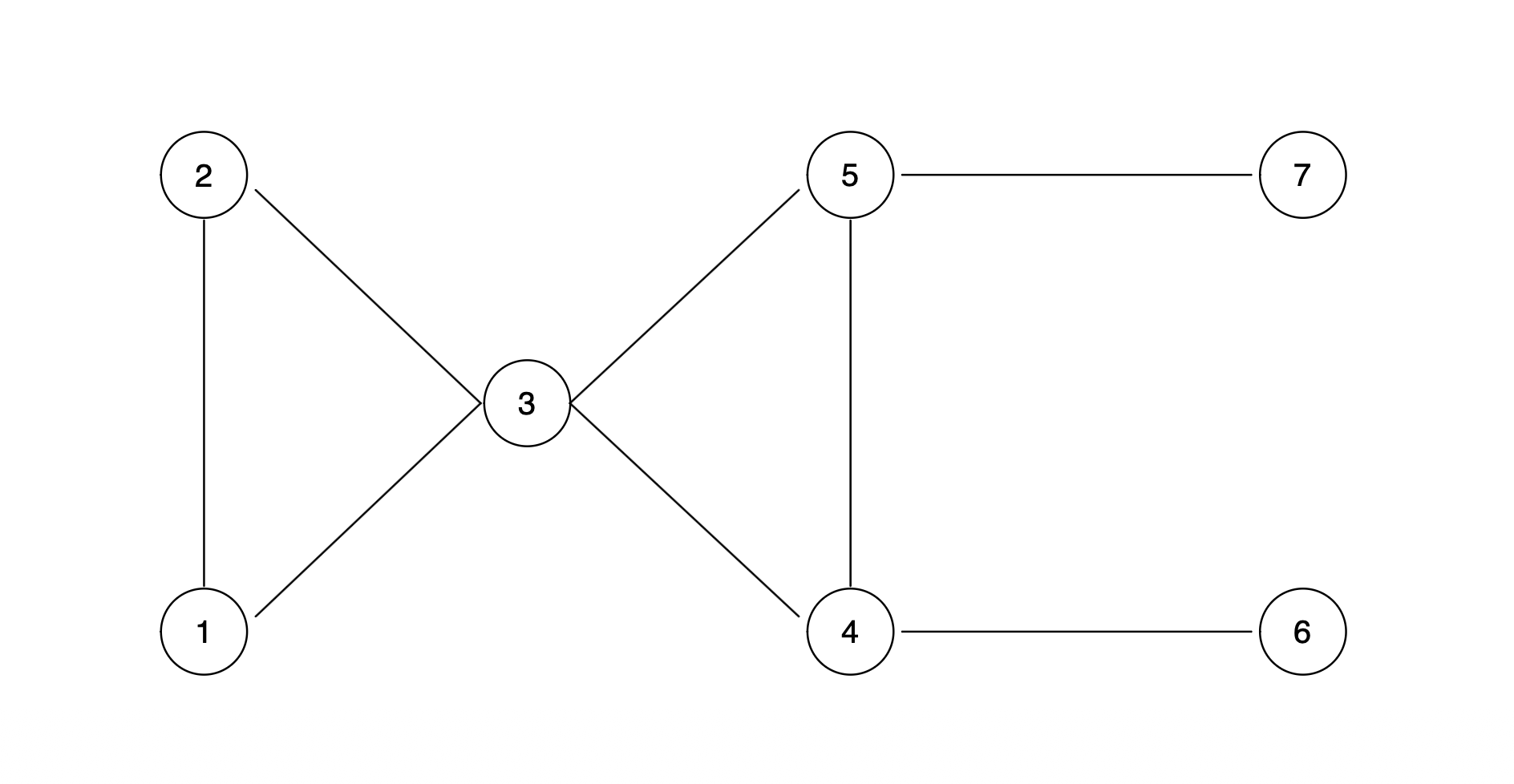
There are 7 random quantities here. We can think of this as a Markov model of sorts, dynamic process where we can transition between these states.
Absence of a line does not mean nodes are independent, it just means they are conditionally independent.
8.2.2 Graphical Models
Conditional independence constraints are simple and interpretable restrictions on joint probability distributions
Conditional independence allows the formalization of the notion of two random quantities being unrelated, given knowledge of a third set of quantities
A Conditional Independence Model is a family of probability distributions that satisfy a collection of conditional independence constraints
It is often convenient to express conditional independence restrictions in terms of a graphoid, i.e. Graphical Models, which summarizes all conditional independence constraints through the algebraic topology of a set of vertices \(V\) and a set of edges \(E\)
8.2.3 Relating a Graphoid to Probability Models
One way to connect a graph \(G = \{V, E\}\) to the distribution of a random vector \(X_V\) is to enforce a certain factorization of the joint probability distribution \(p(x_V)\)
Alternatively, we can connect \(G = \{V, E\}\) to \(p(X_V)\) through a formalization of relationships of conditional independence
We will show through the Hammersely-Clifford Theorem that these two characterizations are essentially equivalent
8.2.4 Factorization over Cliques
- Parametrization of a joint distribution over an UG requires the a suitable modularization of the index set \(V\)
Definition 8.2 (Cliques) Let \(G = \{V, E\}\) be an undirected graph. A clique \(C \subseteq V\) is a collection of nodes, s.t. \((i, j) \in E\) for every \(i, j \in C\).
Definition 8.3 (Maximal Clique) A clique \(C \subseteq V\) is said to be a maximal clique if for any \(v \in V \setminus C\), \(v \cup C\) is not a clique. The set of maximal cliques is denoted as \(\mathcal{C}(G)\)
Define the potential function
\[\psi_C : \mathcal{X}_C \to [0, \infty)\]
A random vector \(X_V\) factorizes according to the graph \(G\) if its density function \(p\) can be represented as
\[p(x_V) \propto \prod_{C \in \mathcal{C}} \psi_C(x_C)\]
The product over cliques can always be restricted to the set of maximal cliques \(\mathcal{C}\)
Sometimes it may be useful to allow for terms not associated with maximal cliques
Example 8.2 (Markov Chains) The standard representation of a Markov Chain is
\[p(x_V) = p(x_1)p(x_2 \mid x_1)p(x_3 \mid x_2) \cdots\]
here we use vertex-based functions \(\psi_j(x_j) = 1\), for \(j > 1\), and \(\psi_1(x_1) = p(x_1)\), combined with the edge wise potentials
\[\psi_{j,j+1}(x_j, x_{j+1}) = p(x_{j+1} \mid x_j), \quad \text{for } j = 1, 2, \ldots\]
The representation above is by no means unique as we could equivalently use the symmetrized potentials \(\psi_j(x_j) = p(x_j)\), \(\forall j\), and
\[\psi_{jk}(x_j, x_k) = \frac{p(x_j, x_k)}{p(x_j)p(x_k)}, \quad \forall (j,k) \in E\]
Example 8.3 (Multivariate Normal Distribution) Consider a vector \(X \sim N_p(0, \Sigma = \Omega^{-1})\), \(\Sigma > 0\) where \(\Omega = \Sigma^{-1}\)
The distribution of \(X\) factorizes as
\[p(x) = (2\pi)^{-p/2}|\Omega|^{1/2} \exp\left\{-\frac{1}{2}x'\Omega x\right\} \propto \exp\left\{-\frac{1}{2}\sum_{(j,k)\in E} \Omega_{jk} x_j x_k\right\}\]
In the Gaussian case the factorization can always be restricted to cliques of size two, even if higher order cliques are present
Example 8.4 (Ising Model) Consider \(X_V \in \{0,1\}^p\), multivariate binary. Given a graph \(G = \{V, E\}\), the ising model defines a joint distribution over \(X_V\), using the following factorization
\[p(x_V) = \frac{1}{Z(\theta)} \exp\left\{\sum_{j \in V} \theta_j x_j + \sum_{(j,k) \in E} \theta_{jk} x_j x_k\right\}\]
8.2.5 Conditional Independence
Definition 8.4 (Conditional Independence) Consider a random vector \(X = (X_1, \ldots, X_p)' \in \mathbb{R}^p\). For any set \(A \subseteq \{1, 2, \ldots, p\}\), let \(X_A = \{X_a\}_{a \in A}\)
Let \(A, B, C \subseteq \{1, 2, \ldots, p\}\) be pairwise disjoint sets. The random vector \(X_A\) is conditionally independent of \(X_B\), given \(X_C\) iff
\[f_{A \cup B \mid C}(x_A, x_B \mid x_C) = f_{A \mid C}(x_A \mid x_C) f_{B \mid C}(x_B \mid x_C)\]
We say \(X_A \perp\!\!\!\perp X_B \mid X_C\)
Proposition 8.1 (Properties of Conditional Independence) Let \(A, B, C, D\) be pairwise disjoint subsets of \(\{1, 2, \ldots, p\}\). The following properties hold:
- Symmetry: \(X_A \perp\!\!\!\perp X_B \mid X_C \Rightarrow X_B \perp\!\!\!\perp X_A \mid X_C\)
- Decomposition: \(X_A \perp\!\!\!\perp X_{B \cup D} \mid X_C \Rightarrow X_A \perp\!\!\!\perp X_B \mid X_C\)
- Weak Union: \(X_A \perp\!\!\!\perp X_{B \cup D} \mid X_C \Rightarrow X_A \perp\!\!\!\perp X_B \mid X_{C \cup D}\)
- Contraction: \(X_A \perp\!\!\!\perp X_B \mid X_{C \cup D}\) and \(X_A \perp\!\!\!\perp X_D \mid X_C \Rightarrow X_A \perp\!\!\!\perp X_{B \cup D} \mid X_C\)
Note: These properties hold for every probability density (w.r.t. any suitable measure)
Definition 8.5 (Intersection Axiom) Unlike the previous four properties, in some special cases, the following holds
Suppose \(f(x) > 0\) for all \(x \in \mathcal{X}\), then:
\[X_A \perp\!\!\!\perp X_B \mid X_{C \cup D} \text{ and } X_A \perp\!\!\!\perp X_C \mid X_{B \cup D} \Rightarrow X_A \perp\!\!\!\perp X_{B \cup C} \mid X_D\]
- This axiom plays a key role in the definition of G-Markov properties and parametrization of joint distributions
- This axiom is holds under strict positivity, but can fail under deterministic restrictions
8.2.6 Undirected Graphs (Pairwise and Local Markov Property)
Let \(G = \{V, E\}\) be an undirected graph
- The probability distribution of \(X_V\) on a graph \(G\) is pairwise Markov wrt. \(G\) if for every pair of vertices \((v, w)\), \((v, w) \notin E\) implies
Considers full edges at a time.
\[X_v \perp\!\!\!\perp X_w \mid X_{V \setminus (v,w)}\]
- The probability distribution of \(X_V\) on a graph \(G\) is local Markov wrt. \(G\) if for every vertex \(v \in V\), we have
Considers one variable at at ime.
\[X_v \perp\!\!\!\perp X_{V \setminus \{v \cup \text{ne}(v)\}} \mid X_{\text{ne}(v)}\]
Lemma 8.1 (Undirected Graphs and Multivariate Gaussian Distributions) If \(X_V \sim N(\mu, \Sigma)\), then the undirected pairwise MP holds iff
\[(v, w) \notin E \iff \Sigma^{-1}_{v,w} = 0\]
The \(v\), \(w\) elements of \(\Sigma\) is equal to 0.
8.2.7 Undirected Graphs (Global Markov Property)
- The Global Markov property is a more general way to formalize conditional independence constraints. We say that the probability distribution of \(X_V\) is global Markov wrt. \(G\) if:
For all \(A, B, C \subset V\), pairwise disjoint, \(A\) and \(B\) nonempty,
\[X_A \perp\!\!\!\perp X_B \mid X_C\]
if \(C\) separates \(A\) from \(B\) in the graph \(G\)
Proposition 8.2 If the distribution of \(X_V\) satisfies the intersection axiom then its joint probability satisfies the pairwise Markov property iff it also satisfies the global Markov property wrt. \(G\).
Example 8.5 (Local vs Global MP) Let \((U, W, X, Y, Z) \in \{0,1\}^5\) be 5 binary random variables with
- \(U \perp\!\!\!\perp Z\) and
- \(p(U=1) = p(Z=1) = p(U=0) = P(Z=0) = 1/2\),
- \(W = U\), \(Y = Z\), \(X = WY\)
The joint distribution over \((U, W, X, Y, Z)\) can be shown to satisfy the pairwise MP wrt. the graph
\[U - W - X - Y - Z\]
Verify that this construction does not satisfy the global MP
8.2.8 Parametrization and Inference
The definition of global MPs for a random vector \(X\) is only useful if a suitable joint distribution \(P(x)\) can be constructed for use in Statistical inference
The availability of a proper joint distribution associated with a graphical model \(G\) relies on two fundamental constructions
- [UG] - Hammersley/Clifford Theorem
- [DAG] - Recursive Factorization Theorem
8.2.9 UG: Hammersely/Clifford Theorem (Besag, 1974)
For all \(C \in \mathcal{C}(G)\), define introduce a continuous potential function \(\psi_C(x_C) \geq 0\), which is a function on \(\mathcal{X}_C\)
The parametrized undirected graphical model consists of all probability distributions on \(\mathcal{X}\) of the form
\[f(x) = \frac{1}{Z} \prod_{C \in \mathcal{C}(G)} \psi_c(x_C)\]
with
\[Z = \int_\mathcal{X} \prod_{C \in \mathcal{C}(G)} \psi_c(x_C) \, d\nu(x)\]
where \(\nu(x)\) is a suitable measure.
Theorem 8.1 A continuous positive probability density \(f\) on \(\mathcal{X}\) satisfies the pairwise MP on the graph \(G\) iff it factorizes according to \(G\).
Example 8.6 (Multivariate Gaussian) Consider \(X \sim N(\mu, \Sigma = K^{-1})\)
The joint distribution of \(X_V\) is
\[f(x) = \frac{1}{Z} \prod_{i=1}^p \exp\left\{-\frac{1}{2}(x_i - \mu_i)^2 k_{ii}\right\} \prod_{1 \leq i < j \leq p} \exp\left\{-\frac{1}{2}(x_i - \mu_i)(x_j - \mu_j)k_{ij}\right\}\]
- Note that the density always factorized into pairwise potentials
- Note that \(f\) satisfies the MP on \(G\) iff for any \((i,j) \notin E\), \(k_{ij} = 0\).
- The original HC construction can be extended to relax the assumption of continuity of \(f(\cdot)\)
- The positivity requirement of the intersection axiom is still required - particularly important when \(X\) is discrete or mixed
Example 8.7 (HC Counterexample) Consider \(X \in \{0,1\}^4\). Assume that the only admitted realizations for this random quantity are
\[(0,0,0,0), (1,0,0,0), (1,1,0,0), (1,1,1,0),\] \[(0,0,0,1), (0,0,1,1), (0,1,1,1), (1,1,1,1)\]
each with probability \(1/8\)
Let \(G\), s.t.
\[G = \begin{array}{ccc} 1 & - & 2 \\ | & & | \\ 3 & - & 4 \end{array}\]
Show that \(f(\cdot)\) is Markov wrt \(G\), but that \(f(\cdot)\) does not factorize according to the HC construction.
8.3 Directed Graphs
8.3.1 Common Types of Graphical Models
Undirected Graphs (Markov Random Fields)
A graph \(G = \{V, E\}\) is an undirected graph if for all pairs \((v, w) \in E\), we have that \((w, v) \in E\). We use the notation \(v \sim w\), whenever \((v, w) \in E\).
Directed Acyclic Graphs (DAGs)
A graph \(G = \{V, E\}\) is directed if \((v, w) \in E\) does not necessarily imply that \((w, v) \in E\). We say \(v \to w\), whenever \((v, w) \in E\). If the graph is directed and the directional paths form no cycles, we say that \(G\) is a DAG.
The literature reports on several other types of graphical models, e.g. reciprocal graphs (Telesca, 2012), chain graphs (Richardson, 2022), \(\ldots\)
8.3.2 Directed Acyclic Graphs (Directed Local MP)
- Directed graphs try to encode a notion of asymmetry in the flow of information along the indices of a random vector \(X_V\)
- Let \(G = \{V, E\}\) be a DAG.
- We say that a probability distribution on \(X_V\) satisfies the directed local Markov Property wrt. \(G\) if, for any \(v \in V\)
\[x_v \perp\!\!\!\perp X_{\text{nd}(v) \setminus \text{pa}(v)} \mid X_{\text{pa}(v)}\]
where
- \(\text{nd}(v)\): set of non-descendants of \(v\)
- \(\text{pa}(v)\): set of parents of \(v\)
8.3.3 Global Directed Markov Property and D-separation
- Let \(G = \{V, E\}\) be a DAG
- Two nodes \(v, w \in V\) are d-connected, given a conditioning set \(C \subseteq V \setminus \{v, w\}\) if there exists an undirected path \(\pi\) from \(v\) to \(w\) such that
- all colliders on \(\pi\) are in \(C \cup \text{an}(C)\), [\(\text{an}(w)\) = set of ancestors of \(w\)]
- no non-collider on \(\pi\) is in \(C\).
- Let \(G\) be a DAG. The distribution of \(X\) wrt \(G\) satisfies the directed global MP if, for all pairwise disjoint triplets \(A, B, C \subseteq V\), \(A\) and \(B\) nonempty,
\[A \perp_D B \mid C,\]
i.e. \(C\) d-separates \(A\) and \(B\)
8.3.4 Recursive Factorization for DAGs
Let \(X_V\) be a random vector
We say that \(p(x_V)\) is Markov wrt. a DAG \(G = \{V, E\}\) iff
\[p(x_V) = \prod_{j \in V} p(x_j \mid \text{pa}(x_j))\]